Module 10 Supervised Classifiction

Module 9 Unsupervised Classification

For this week in Remote Sensing we explored unsupervised classification of features, using both ArcMap and ERDAS.  The map above depicts five separate feature classifications.  To create this map we first took a provided image and created another image with 50 classifications.  Once this was complete, we then reclassified the image into just five classifications; this was all done in ERDAS.  To make the final map I used ArcMap and added all the map essentials.

Module 8 Thermal and Multispectral Analysis

In Module 8 we created composite images and continued exploring histograms, breakpoints, and band combinations to better understand and view features. In this module we were task with locating a feature of interest within a given image and creating a map, using the skills gained in this module to display the feature on a map. The map above depicts Test Range B-70 located on Eglin, AFB in Florida.

Module 7 Multispectial Analysis

For this module in Remote Sensing we were to identify certain features of an image based on their pixel count in certain layers.  This was accomplished using the image histogram and the inquire cursor tool.

In layer four there was a spike between pixel values 12 and 18. This was on the left side of the histogram, and from the module I knew this would mean a dark area of the image.  From the image it appeared this may be deep water. Using the search cursor I verified that there was a correlation between pixels in the histogram and the area I had selected on the image.  Once this was done I used the Inquire box and the Subset & Chip tool to select an area that best depicted this feature in the image and saved this as new file. I then opened the file in ArcMap and created the map above.

In layers 1-4 there was a small spike around pixel value 200 and a large spike between pixel values 9 and 11 in layers 5 and 6. This was on the right side of the histogram, and from the module I knew this would mean a very light area of the image.  From the image it appeared this may be the snowcapped mountains. Using the search cursor I verified that there was a correlation between pixels in the histogram and the area I had selected on the image.  Once this was done I used the Inquire box and the Subset & Chip tool to select an area that best depicted this feature in the image and saved this as  a new file.  I then opened the file in ArcMap and created the map above.

  

 

 

 

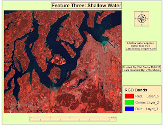
In certain areas of the water, layers 1-3 are much lighter than normal.  Layer 4 was a little brighter and layers 5 and 6 were unchanged. From the image it appeared this may be several areas of shallow water. Using the search cursor I verified that there was a correlation between pixels in the histogram and the area I had selected on the image.  Once this was done I used the Inquire box and the Subset & Chip tool to select an area that best depicted this feature in the image and saved this as a new file. I then opened the file in ArcMap and created the map above.

 

 

Module 6 Spatial Enhancement

 

 

 

Week 6 of Remote Sensing covered Spatial Enhancement.  In this module we covered various methods used to enhance imagery. The map above is the result of starting with a LandSat image and using the convolution tool to enhance the image, using the trial and error method; I finally decided that using the 3x3Sharp5 filter worked best to remove the striping and still keep the image somewhat identifiable.  I am sure that with more experience I could do a better job, but for now this is the best I could come up with.  

  

Intro to ERDAS Imagine and Digital Data

Week 5 of Remote Sensing covered the basics of ERDAS Imagine.  For this module we were given an opportunity to explore where some of the tools were located and how to use them. We also used the viewer to view data in ERDAS Imagine.  We then preprocessed an image for making a map in ArcGIS. I am however a little leery because the lab instruction mentioned “crashes” and using “work arounds” to make ERDAS Imagine work properly.    But with that said, I was able to create the map above without much problem.  The map depicts a sub-section of an image of forested area in Washington state which was classified into different types of ground cover.  

Ground Truthing and Accuracy Assessment

Module 4 of Remote Sensing, covered Ground Truthing and Accuracy Assessment.  For this project we used the LULC map from last weeks module, and since actually going to the site and verifying the accuracy of our LULC assessment was not feasible, Google maps street view was used.  First I selected 30 random points within the study area. Then using Google maps I located these exact points, and zooming to the street view I was able to verify if, in fact, my assessment of that particular point was correct.  Once this was complete I calculated the overall accuracy of LULC Assessment.  In this case, of the 30 points that were checked, three were found to be incorrectly identified resulting in an overall accuracy of 90%.  

LULC Classification

Module three of my Remote Sensing course covered Land Use and Land Cover Classification.  Given a aerial photograph of the Pascagoula, Mississippi area I created a shape file of polygons that depict different land uses and land covers. This was done only to the second level as shown in the legend.  Techniques and criteria used to identify these areas were covered in Module two. 

Interpreting Aerial Photographs

Above are two maps I created using aerial photographs. The first map shows several features I was able to identify using four sets of criteria; Shape and Size, Shadow, Pattern, and Association. In the second map I selected five areas showing separate textures, and five areas with show five separate tones.